 Learn AI
Load data you can trust.
A shuffled file can silently attach the wrong answer to every example. Inspect the join, reproduce the transformation, then write a loader that refuses ambiguous input.
This P02 studio covers CSV contracts, NumPy arrays, an isolated environment and real-data plots. The browser preview needs no installation. Runnable implementation evidence requires Python 3 and your own code. This optional work does not change guided completion or award mastery. Human review and learner pilots remain pending.
Enter here, or refresh one idea
Know what a list, loop and function do. A CSV is a text table: its first line names the columns. A schema is the agreement about those names and values. A join matches records by a shared ID, not their location in a file.
Practice programming first · Refresh splits, units and leakage · See target pairing in neural training. Already comfortable? Skip directly to the coding task and supply equivalent evidence.
Try → predict → experiment
Four synthetic rows represent different measurement groups. The input file has IDs a, b, c, d. A separate target file arrives in order d, c, a, b with targets 8, 2, 1, 3. These are teaching values, not the Iris data or model predictions.
Inspect a live loading trace
First try both faults separately. Then restore both controls. Predict whether changing only the evaluation input should change the training mean.
- Read named columns
- Convert a: 10 mm ÷ 10 = 1 cm
- Match target IDs
- Fit training rows only
- Fill and transform every row
Fitted mean: 2.0000 cm. Population standard deviation: 1.0000 cm. Changing evaluation input leaves the fitted transformation unchanged.
| Input ID / split | Input cm | Target ID → value | ID check | Filled cm | Standardized |
|---|---|---|---|---|---|
| a / training | 1 | a → 1 | Matched | 1.0000 | -1.0000 |
| b / training | 3 | b → 3 | Matched | 3.0000 | 1.0000 |
| c / development | missing | c → 2 | Matched | 2.0000 | 0.0000 |
| d / evaluation | 8 | d → 8 | Matched | 8.0000 | 6.0000 |
Preview settings are temporary. No files are uploaded and no learner code runs here.
Understand the numbers
The two training values are 1 and 3 cm. Their mean is (1 + 3) ÷ 2 = 2 cm. Their distances from that mean are −1 and 1 cm. Square those distances, average them, then take the square root: √((1 + 1) ÷ 2) = 1 cm. This is the population standard deviation used by this exercise.
For each value x, calculate z = (x − μ) ÷ s. Here μ (mu) is the stored training mean and s is the stored training standard deviation. Read this as “distance from the training mean, measured in training spreads.” Thus 8 cm becomes (8 − 2) ÷ 1 = 6. Missing measurements use μ before the transformation. A constant training column uses divisor 1 and an explicit flag; no observed training measurements is an error.
Filling before computing the standard deviation matters when training values are missing. The loader uses the observed training mean, fills missing training values with it, and then computes the spread of that filled training column. This is a declared teaching policy, not a universally appropriate missing-data strategy.
Apply: run, complete, break, repair
Download Python data-loader starter
- Save the file in a new folder. Run
python3 data-loader.py --demo. Inspect the supplied trace: the demo uses a supplied join and does not run your unfinished function. - Implement
join_targets. Build an ID lookup, reject missing/extra/duplicate IDs, convert finite target numbers, and return new records in input order. Do not mutate the supplied rows. - Run
python3 data-loader.py --check. Until you implement the function, the tests intentionally fail with a TODO error. These visible cases are development feedback. - Create the two files below and run
python3 data-loader.py --csv measurements.csv --labels targets.csv. Redirect output to a new report file if desired. The report includes byte counts and SHA-256 hashes identifying the exact input bytes; a hash does not establish a source's trustworthiness. - Reorder columns, add an unused notes column containing a quoted comma, shuffle labels and confirm that the output remains equivalent. Then duplicate an ID and move one group across partitions: each must be rejected.
Copyable synthetic CSV files
measurements.csv
id,group,split,length,unit
a,A,training,10,mm
b,B,training,3,cm
c,C,development,,cm
d,D,evaluation,80,mm
targets.csv
target,id
8,d
2,c
1,a
3,b
Required input columns: id, group, split, length, unit. Split is training, development or evaluation; length may be blank; unit is cm or mm even when missing. Target columns: id and target; targets cannot be missing. Columns may be reordered and extra columns are ignored by the transformation. Each file is capped at 100,000 bytes and 1,000 records. Numeric magnitude before unit conversion is at most 1,000,000. Group names must be meaningful for your intended evaluation: validating supplied names does not prove real-world independence.
Arrays: preserve the meaning of each dimension
NumPy stores a rectangular collection of values in an array. Shape (89, 4) means 89 examples and four features. A float64 stores a floating-point number using 64 bits; arithmetic is approximate, so tests use a tolerance. Axis 0 is the row direction and axis 1 is the column direction. A slice may share storage with its parent: use .copy() when you need an independent experiment.
Which direction should the mean collapse?
Columns are two measurements in cm; rows are examples. Predict the result, then change the reduction axis. This preview implements the displayed arithmetic; NumPy runs only in the downloaded Python exercise.
X · shape (2, 2)
| Feature A | Feature B |
|---|---|
| 1 | 10 |
| 3 | 30 |
mean · shape (2,)
[2, 20] cm
One mean per feature: suitable for centering each column.
X − mean
| -1 | -10 |
| 1 | 10 |
Each column is centered around its own training mean.
axis=0 reduces the row direction. For the two-row case, Feature A's mean is (1 + 3) ÷ 2 = 2; Feature B's is (10 + 30) ÷ 2 = 20. Broadcasting repeats these two values for each row without making them new fitted statistics.
Temporary practice. No saved evidence or mastery is awarded.
Create an isolated environment
Use Python 3.11 or newer for this optional exercise. A virtual environment keeps its packages separate from other projects. The commands below invoke that environment's interpreter directly, so activation is optional. The browser course remains available without installing anything. Package installation needs an internet connection; the downloaded exercise and dataset run locally afterward.
Download array inspection exercise · Download pinned direct dependencies · Download Iris CSV · Download provenance manifest · Download attribution
macOS or Linux commands, from a new exercise folder
python3 -m venv .venv
.venv/bin/python -m pip install -r studio-requirements.txt
.venv/bin/python array-inspection.py --csv iris.csv --out inspection-01
.venv/bin/python -m pip freeze > environment-freeze.txt
Windows PowerShell commands
py -3 -m venv .venv
.venv\Scripts\python.exe -m pip install -r studio-requirements.txt
.venv\Scripts\python.exe array-inspection.py --csv iris.csv --out inspection-01
.venv\Scripts\python.exe -m pip freeze > environment-freeze.txt
Direct dependencies are pinned to NumPy 2.3.5 and Matplotlib 3.10.8, verified here with Python 3.12.14 on macOS ARM64. The freeze file records installed transitive versions too; keep it alongside your OS and Python version. It is a reproducibility record, not a promise that binary packages install on every platform. If installation fails, read the package error and continue with the browser trace while resolving the environment.
Inspect before learning
The supplied run creates a new output folder containing report.json, development.csv, inspection.png and a caption/attribution file. It refuses an existing output directory. The report contains exact CSV hash/size, array shapes, training means/scales and environment versions. This supplied path is explicitly labelled; it is not evidence that you implemented the transform.
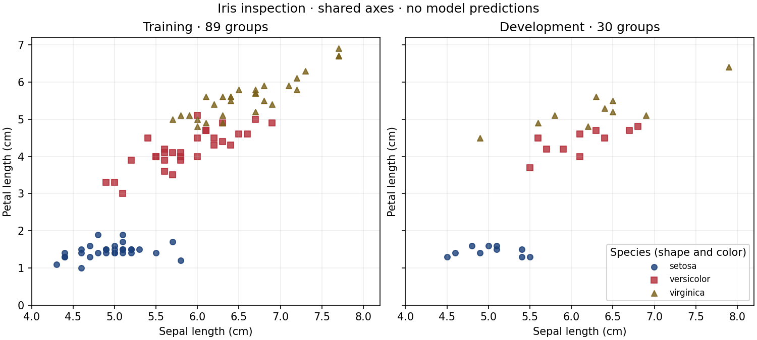
Iris has four measurements in cm. One duplicate measurement vector is removed, leaving 149 groups. Within each species, deterministic first-occurrence group indices modulo five allocate 89 training, 30 development and 30 evaluation groups. This studio split is distinct from the original two-way feasibility manifest. Generated row IDs are not specimen IDs, and equal measurement vectors do not prove specimen identity. This public dataset has appeared in earlier lessons: reserved membership here does not mean previously unseen.
The two scatter panels compare sepal length with petal length on identical axes. Species differ by both shape and color. The accompanying CSV provides numerical values; the plots show measured relationships, not model predictions. No classifier is fitted and no final evaluation score or evaluation scatter is produced.
Complete → repair → transfer
- Open the report: confirm train shape (89, 4), development shape (30, 4) and float64 dtype. Match one plotted point to its raw measurement row.
- Implement
learner_standardize: validate shapes and finite values, fit mean and population spread per training column, use divisor 1 for constant columns, and transform development with those same values without editing either input. - Run
array-inspection.py --checkwith your environment's Python. The TODO deliberately fails until implemented. Then run with--learner --csv iris.csv --out inspection-02and compare results with the supplied artifact. Shape checks alone do not prove the arithmetic correct. - Introduce
axis=1. Explain why a square example can run with wrong meaning while a rectangular example fails. Repair it and add a three-row, two-feature test. Perturb development values and verify that training means/scales do not change. - Change the supplied plot to compare sepal width and petal width. Update both axis labels and choose shared limits containing all shown points. Include a numerical alternative and explain why visual separation is not held-out predictive performance.
- Have a reviewer supply a different CSV column order and array shape, including a constant feature. Reproduce the report from a fresh environment. Keep the review pending until that actually happens.
Source: Fisher, R. (1936), Iris, UCI Machine Learning Repository, CC BY 4.0. The local asset adds headers and generated IDs; original measurements and labels are unchanged. Explain a different dataset's source, permission and missing-data policy before adapting this exercise.
Further reading: NumPy array basics, Python virtual environments, and Matplotlib plotting guide.
Evidence for different goals
- Understand: explain one wrong join and calculate the transformed missing row. Predict what changes if only evaluation data changes.
- Implement: submit your runnable function, input files, commands, output and tests. Add cases for constant/all-missing training values and shuffled columns. A reviewer must supply a genuinely new file shape and check the reasoning; passing visible tests alone is not independent proficiency.
- Decide: write a short acceptance brief: which schema failures block loading, who owns group definitions, why source permission matters, and what the report cannot establish about a model.
Keep artifacts locally. This studio does not yet save a draft or review record in My Work. Human artifact review remains pending.
Use this evidence in the data audit project · Continue to P03 classical ML pipelines · Return to Explore